Prototyping – Part I

Well I finally got around to get some code and test things out. Without known test loads and an oscilloscope, testing shall require some creativity.  Armed with a multimeter I began testing things out.

Software

The longer term plans include creating spot measurement devices  using the arduino and rather than slapping the code and copying and pasting stuff around, I opted to create a couple of classes to facilitate reuse. It took some trial and error to understand how to add classes to the arduino dev environment and could never get multiple inheritence to compile in the environment. I assumed the problem was between the keyboard and the chair.

I ended creating two classes: ACSignal to help capture and compute some basic stuff like average, RMS values. The PowerSignal class takes two ACSginal references and computes apparent power, real power, etc.

The code to use the classes is rather simple. Converting the float to alpha–since the LCD4Bit library does not handle spitting out floats–took more time that I wanted.

As explained earlier, the math looks more complicated than it is. The two main formulas are shown below along with the corresponding code to implement it. Anti-climatic if you ask me, but nice to see the stuff working.  As long as the sampling rate is much greater than the highest frequency component, things should be good to go. I take 2000 samples display stuff and resample.  Since this is all this arduino does I don’t need interrupt driven sampling periods. The maximum sampling rate for the ATMEGA chip on the arduino is around 9600 hz.  More than enough for this power line sampling.

P_{avg} = \frac{1}{N}\sum_{n=1}^{N}v_ni_n \approx \frac {1}{T}\int^{to+T}_{to}p(t)dt \qquad(1) X_{rms}= \sqrt{\frac{1}{N}\sum_{n=1}^{N}x^2_n} \approx \sqrt{\frac {1}{T}\int^{to+T}_{to}x^2(t)dt} \qquad(2)

@@

void PowerSignal::updateAccumulator()
{
  mSumVoltageTimesCurrent += mVoltageSignal.getInstantaneousValue() * mCurrentSignal.getInstantaneousValue();
}

float PowerSignal::computeAveragePower()
{
 return( mSumVoltageTimesCurrent / mVoltageSignal.getSampleCount() );
}

float ACSignal::acquireSignalSample()
{
 float lVal;

 mCurSample = analogRead( mPin )  ;
 mCurVoltage = mCurSample * PS_VOLTS_PER_STEP;
 mSampleCount++;
 mSumVoltageRaw += mCurVoltage;
 mRealVoltage = mCurVoltage - mDCOffset;  // remove DC offset from circuit voltage divider
 lVal = getInstantaneousValue();
 mSumVoltageSquared +=  lVal * lVal;

 if( lVal > mMax )
 mMax = lVal;

 if( lVal < mMin )
 mMin = lVal;

 return( lVal );

}
float ACSignal::getRMSValue()
{
 float lRMSValue = PS_PWR_CALC_ERR;
 if( mSampleCount > 0 )
   lRMSValue = sqrt( mSumVoltageSquared / mSampleCount );
 return( lRMSValue );

}

Discrete Time Equivalents

Earlier I spoke about modeling the math to simulate the calculations that I will be using in my home grown energy monitoring system. I think I have a good enough grasp on the math to come up with the algorithm to use in the software. Specifically, the computation of RMS values and average power.

P_{avg} = \frac{1}{N}\sum_{n=1}^{N}v_ni_n \approx \frac {1}{T}\int^{to+T}_{to}p(t)dt \qquad(1) X_{rms}= \sqrt{\frac{1}{N}\sum_{n=1}^{N}x^2_n} \approx \sqrt{\frac {1}{T}\int^{to+T}_{to}x^2(t)dt} \qquad(2)

The simulation implemented both these and the integration functions to compare results. We are dealing with low frequency power line signals of 60hz which in theory we need to sample at 120 times per second. The reality is that there will be higher frequency components such as harmonics and we would need to sample at a higher rate capture those effect and ensure we can compute true RMS values.

Don Lancaster’s Tech Musings provides an excellent summary about measuring power s and pitfalls in trying to measure it.

I think I have enough theory and now ready to start building something.

Modeling the Math

I used Excel to enter the power calculations on a simulated data set (voltage and current). I later wanted something more responsive to what-ifs and designed for mathematical computation. I stumbled on a MatLab like open source tool cal GNU-Octave. I decided to download and install the tool to enter basic power calculations.

What I like about this tool and like Matlab is the ability to manipulate matrices and vectors. I can set up calculations for my power without resorting to annoying for loops. With my short attention span, I liked this.

Earlier I described the basic math and reduced the following salient equations:

P_{avg}=\frac {1}{T}\int^{to+T}_{to}p(t)dt\qquad(1) I_{equiv}=I_{rms}=\sqrt{\frac {1}{T}\int^{to+T}_{to}i^2(t)dt} \qquad(2) P_{avg} = V_{rms}I_{rms}cos(\Theta_v-\Theta_i) \qquad(3))

For giggles, I wanted to use Octave to calculate and plot power curves. I know from sampling theory that we need to sample at least at the Nyquist frequency to be able to reconstruct the signal.The reality is we don’t live in an ideal world with perfect filters. More about sampling rate later.

I created functions in Octave to generate a waveform. I can also import a text file with data values and compute the various types of powers as well. I wanted to test a couple of sunny day scenarios to ensure that my calculations were correct. I took two approaches. One I actually defined the function and let Octave integrate it. The other was to sample the function like I would in the software. Both yielded the same results. The table below outlines the expected and actual results.

Package/ToolURLDescriptionInstallation
log4jslog4jslog4js based logging services for node.jsnpm install log4js -S
monkmonkwrapper to mongodb that is simpler yet not as powerful as mongoosenpm install monk -S
nodemonnodemonlistens for file changes and restarts server npm install nodemon -g
dummy-jsondummy-sontool to generate JSON files used for my testingnpm install dummy-json -g
RobomongorobomongoMongoDB managerdownload and point to mongoDB instance (default localhost:27017)
Bluebirdbluebirdpromise library implementationnpm install bluebird -S
SerialPortserial portserial port driver for node.jsnpm install serialport -S # have 4.0.7
xbee-apixbee-apixbee API for node.jsnpm install xbee-api -S

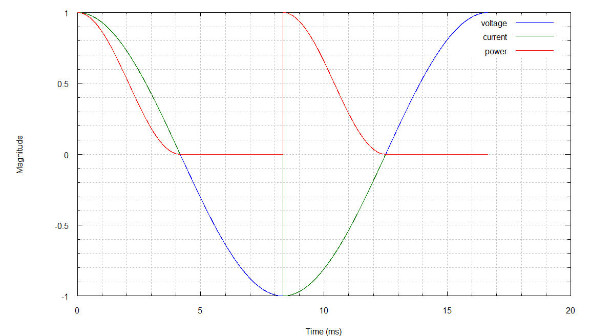
I also generated an odd current waveform that could occur in speed control via a triac or something and ploted the graph below.

SCR

Intuitively one would expect the average power to be half of the sunny day scenario. The other half is reactive power. The following shows the power calculations for varying sampling rates.

[table “3” not found /]