Discrete Time Equivalents

Posted on November 21, 2009 by Peter Chrapchynski

Earlier I spoke about modeling the math to simulate the calculations that I will be using in my home grown energy monitoring system. I think I have a good enough grasp on the math to come up with the algorithm to use in the software. Specifically, the computation of RMS values and average power.

$P_{avg} = \frac{1}{N}\sum_{n=1}^{N}v_ni_n \approx \frac {1}{T}\int^{to+T}_{to}p(t)dt \qquad(1)$ $X_{rms}= \sqrt{\frac{1}{N}\sum_{n=1}^{N}x^2_n} \approx \sqrt{\frac {1}{T}\int^{to+T}_{to}x^2(t)dt} \qquad(2)$

The simulation implemented both these and the integration functions to compare results. We are dealing with low frequency power line signals of 60hz which in theory we need to sample at 120 times per second. The reality is that there will be higher frequency components such as harmonics and we would need to sample at a higher rate capture those effect and ensure we can compute true RMS values.

Don Lancaster’s Tech Musings provides an excellent summary about measuring power s and pitfalls in trying to measure it.

I think I have enough theory and now ready to start building something.

Modeling the Math

Posted on November 17, 2009 by Peter Chrapchynski

I used Excel to enter the power calculations on a simulated data set (voltage and current). I later wanted something more responsive to what-ifs and designed for mathematical computation. I stumbled on a MatLab like open source tool cal GNU-Octave. I decided to download and install the tool to enter basic power calculations.

What I like about this tool and like Matlab is the ability to manipulate matrices and vectors. I can set up calculations for my power without resorting to annoying for loops. With my short attention span, I liked this.

Earlier I described the basic math and reduced the following salient equations:

$P_{avg}=\frac {1}{T}\int^{to+T}_{to}p(t)dt\qquad(1)$ $I_{equiv}=I_{rms}=\sqrt{\frac {1}{T}\int^{to+T}_{to}i^2(t)dt} \qquad(2)$ $P_{avg} = V_{rms}I_{rms}cos(\Theta_v-\Theta_i) \qquad(3))$

For giggles, I wanted to use Octave to calculate and plot power curves. I know from sampling theory that we need to sample at least at the Nyquist frequency to be able to reconstruct the signal.The reality is we don’t live in an ideal world with perfect filters. More about sampling rate later.

I created functions in Octave to generate a waveform. I can also import a text file with data values and compute the various types of powers as well. I wanted to test a couple of sunny day scenarios to ensure that my calculations were correct. I took two approaches. One I actually defined the function and let Octave integrate it. The other was to sample the function like I would in the software. Both yielded the same results. The table below outlines the expected and actual results.

Package/Tool	URL	Description	Installation
log4js	log4js	log4js based logging services for node.js	npm install log4js -S
monk	monk	wrapper to mongodb that is simpler yet not as powerful as mongoose	npm install monk -S
nodemon	nodemon	listens for file changes and restarts server	npm install nodemon -g
dummy-json	dummy-son	tool to generate JSON files used for my testing	npm install dummy-json -g
Robomongo	robomongo	MongoDB manager	download and point to mongoDB instance (default localhost:27017)
Bluebird	bluebird	promise library implementation	npm install bluebird -S
SerialPort	serial port	serial port driver for node.js	npm install serialport -S # have 4.0.7
xbee-api	xbee-api	xbee API for node.js	npm install xbee-api -S

I also generated an odd current waveform that could occur in speed control via a triac or something and ploted the graph below.

SCR

Intuitively one would expect the average power to be half of the sunny day scenario. The other half is reactive power. The following shows the power calculations for varying sampling rates.

[table “3” not found /]

Steady State Power Analysis

Posted on November 16, 2009 by Peter Chrapchynski

I wanted to brush up on the theory before I jump to the implementation. So back to basic circuit analysis.

Instantaneous Power
In a steady state system, the voltage and current as a function of time consists of

$v(t)=V_{max}cos(wt + \Theta_v) \qquad(1)$ $i(t)=I_{max}cos(wt + \Theta_i) \qquad(2)$

where $\Theta_x$ is is the phase angle of the voltage and current respectively

The instantaneous power is defined as
$p(t)=v(t)i(t)=V_{max}I_{max}cos(wt + \Theta_v)cos(wt + \Theta_i)\qquad(3)$

Using some trigonometry, (3) reduces to
$p(t) = \frac{V_{max}I_{max}}{2}[cos(\Theta_v-\Theta_i) + cos(2wt + \Theta_v + \Theta_i)]\qquad(4)$

(4) shows that the instantaneous power has a constant or DC component and a time-variant component and illustrated below. (v=1, i=1, $\Theta_v=\Theta_i=0$ )

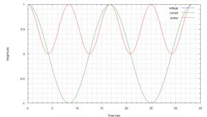
Note the average component “the DC offset” and the frequency of the instantaneous power is two times that of the voltage or current.

We can compute the average power by integrating (4) over one period. We get

$P_{avg}=\frac {1}{T}\int^{to+T}_{to}p(t)dt\qquad(5)$

If one substitutes (4) into (5), (5) reduces to $P=\frac{1}{2}V_{max}I_{max}$ in a purely resistive circuit and $P=\frac{1}{2}V_{max}I_{max}cos(90^\circ)$ assuming a sinusoidal waveform.

RMS Values
In the power measurement solution for home, one can assume purely resistive loads and sinusoidal voltages and currents. That will come at the price of accuracy. The reality loads such as computers, UPS, etc. introduce inductance and capacitance which create loads that are neither purely resistive nor purely reactive. Furthermore, the current and voltage profiles are not clean sine waves.

Recall that the average power absorbed by a purely resistive load using a sinusoidal source was $P_{avg}=\frac{1}{2}V_{max}I_{max}$ . Note that if the source was a DC, then $P_{avg}=I^2R$ What if the source is not a sinusoidal wave? Is there an equivalent constant current that can be computed that delivers the same average power to a purely resistive load (R)? .e.g. $P_{avg} = I^2_{equiv}R =\frac {1}{T}\int^{to+T}_{to}i^2(t)Rdt$ solving for $I_{equiv}$ we get

$I_{equiv}=I_{rms}=\sqrt{\frac {1}{T}\int^{to+T}_{to}i^2(t)dt} \qquad(6)$

Plug in in a sinusoidal current like $i(t)=I_{max}cost(wt + \Theta)\quad T=\frac{2\pi}{w}$ into (6) we get the infamous $I_{rms}=\frac{I_{max}}{\sqrt{2}}$

Given this view of the RMS current, one can write the average power as

$P_{avg} = V_{rms}I_{rms}cos(\Theta_v-\Theta_i) \qquad(7))$ In the North-American 120 volt system, the 120 is the RMS voltage and $V_{max} = 120\sqrt{2}\approx 170V$

For non-sinusoidal functions, more complex integration needs to occur. Fortunately, in the implementation, there are some assumptions we can make to approximate the integration that makes the math much simpler. Nevertheless, an understanding of the math is needed to bend the rules.

Power Factor
One last component needs to be addressed and that is the power factor. Equation (7) contains two components. The product of $V_{rms}I_{rms}$ is known as the Apparent Power (S) and the $cos(\Theta_v-\Theta_i)$ as the Power Factor.

In an purely resistive circuit, $P_{avg}=P_{apparent}$ since $cos(\Theta_v-\Theta_i) = 1$

Moving Forward

The reference implementation shall compute the average power, Irms and Vrms. Using (7), one can compute the power factor. e.g. $\frac{P_{avg}}{V_{rms}I_{rms}} = PF$

The power factor angle = $arccos{\frac{P_{avg}}{V_{rms}I_{rms}}}$ The reactive power can be computed by the relation $S^2 = P^2_{avg} + Q^2$ where Q is the reactive power in vars. Solve for Q and we can now compute all power related components.

Now you may ask why the Power Factor Angle? We don’t even reference it? Well, you could use to compute the reactive power. What it does give me is sense of the types of loads I have in the house. A value closer to 0, implies I am operating in a resistive load. If you look at the power factor angle of a variable speed drill, at low speeds the angle would be far from zero. At full RPM the angle would approach zero. Why this is the case is because how variable speed drills work. That is a separate discussion.

Next I want to model the math using a tool to help me make some assumptions for my reference implementation.

Ponderings

Musings of a Tech Minimilist

Category Archives: Math

Discrete Time Equivalents

Modeling the Math

Steady State Power Analysis